Learning markov chains
This post describes my recent effort to learn about markov chains. I had worked with markov chains only very superficially before and was not at all comfortable with them; in particular, it would have been hard to think of using them to solve real-world problems.
More generally, this is part of my effort to implement a consistent learning process for myself - to create a study habit. I expect that to be a requirement for me to develop professionally as a data scientist.
I’ll focus on two sides of this effort. First of all, I’ll describe the process I followed to implement a learning habit and why I think that is important. I’ll also highlight some key points that worked for me. The goal here is to have a summary of the learning process that I can revisit later and iterate upon. Secondly I’ll put forward a summary of what I learned about markov chains. The goal here is for me to be able to come back to this in a couple months and refresh my memory on the subject.
Part 1: Process
What’s the point of a learning habit?
There’s plenty of support for the idea that creating a habit around some activity is the best way to do it consistently, and it is also consistent with my own personal experience, so I assumed this hypothesis. I had previously tried to start personal free-time projects around learning or exploring some interesting question, and the roadblock I always got stuck on was my inability to put in the hours that the project required. I would typically start out very excited, finding lots of time to play around with the main idea, and after some time the enthusiasm would fade and the project would be left unfinished.
So what I wanted to do was find a way of fitting a couple of hours a week into my schedule in a way that would allow me to put in the hours as effortlessly as possible. This is the point of forming a learning habit: to allow myself to have some regular amount of time to work on, develop or explore whatever I think is important at that time (in other words, finding time for Q2 in the Eisenhower matrix).
What process did I implement and how did it work?
The first thing I did when I decided to give this a meaningful try was to reach out to a friend to discuss my goals and strategy and ask for his support. This resulted in immensely helpful input on how to go about creating this habit as well as regular discussions which were essential for sticking to it. While I don’t expect this to be universally true, attempting this process without someone actively involved in it would have been much harder and probably unsuccessful.
Here’s what we ended up implementing:
-
we set regular working hours. 3 pomodoros per weekday before work (from 6:15 to 7:45) and 5 pomodoros on saturday morning (no set hours, but first thing), resulting in 10 hours a week.
-
we set up a shared spreadsheet for keeping track of progress. This was a simple spreadsheet with 2 rows per week, one for planned hours and one for executed hours, and a column for every day (plus some room for comments for each week). Crucially, we set it up so that days when I put in the expected hours showed up in green, whereas days when I did not showed up in red. This led to the concept of green weeks which I discuss below.
-
we set up weekly discussions. These were typically half to one hour talks on last week’s progress and next week’s plan, usually on sundays. I see these discussions as the glue to the whole process: they kept me accountable on a weekly basis, which made it very uncomfortable to accept underperforming weeks; they allowed me to reflect on what I had learned the past week; and they steered next week’s efforts.
This implementation is not set in stone but it is what we are currently rolling with. We arrived at it after trying some variations and learning from them. Some points I think were important for me to become aware of:
-
deviating from routine is the most difficult thing to adjust to. I found that if I could not work at all in the mornings, as planned, it became very difficult to start working later in the day (this is not the same as working in the morning but not being able to finish). This was very relevant when travelling or taking some days off, which I felt disrupted my plan very much - more than just the net effect of the days missed. As a solution for this I think it’s best to plan ahead and simply not plan any work in days where I don’t expect to be able to do them as I would regularly.
-
whenever I failed to put in the planned pomodoros for any given day, I had as a rule to put in the missing amount plus one on any other day. This provided a helpful extra incentive to put in the planned hours each day. Right now, if for some reason I cannot work the full time in the morning, I manage to do it later in the day instead, and I think this rule was helpful in achieving that.
-
I needed a rest day. I started out very ambitiously with planned pomodoros every day, and that failed very fast. Eventually I settled on leaving sunday free. This, coupled with working saturday mornings, resulted in a pleasant feeling of accomplishment which allowed me to start enjoying weekends in a calmer, stress-free manner which I hadn’t experienced for a long time.
Some concerns I still have to solve is how to deal with saturday’s extra work (5 pomodoros instead of 3), which makes it more difficult to start working, and also how to handle resting (as in, stop for one week every once in a while). I think these will be important long-term, but for now the present approach has worked pretty well.
Key highlights
I found three factors that contribute mightily to being able to sustain a learning habit:
- green weeks
- regular feedback
- tangible artifacts in the end
By green weeks I mean literally seeing the color green in the spreadsheet, as a result of actually putting in the hours for the entire week. I felt that after seeing green for one or two weeks it became very hard to accept a red week, which meant that accomplishing the day’s goal became my primary concern, which in turn made it a lot easier to start working, keep working, and going back to work in case the goal had not been accomplished in the morning.
By regular feedback I mean talking to a person about your project on some periodic, well-defined basis, e.g. once a week. It is important that this person is aware of your project, your goals and your progress, for example through access to the spreadsheet. Although it helps, I don’t think it is necessary for that other person to be technically knowledgeable or to even be able to point you in the right direction. What is crucial is to feel accountable towards that person and therefore feel embarassment for not achieving the planned weekly goals. I found this was a powerful motivation and helped me avoid distraction and procrastination.
Finally, I think it is important to have as a final goal something tangible - something material, with physical existence that can be shown to other people or just yourself. This blog post is this project’s tangible goal. I thought this helped on two accounts: it kept me more focused during the learning process than I would have been otherwise, and it provided a sense of accomplishment upon completion of the project. Hopefully it will also be useful in the future, if I need to review or re-learn these contents - but it is important even if I never look at markov chains again.
Part 2: Markov chains
What I set out to learn
I had two key goals for this process. First was establishing a learning habit and second was learning some subject that I thought was both interesting and useful. I decided to pick up Markov chains for a couple of reasons:
-
it is a topic that recurrently pops up on my radar.
-
as far as I could understand, it was fairly simple and self-contained (meaning there were no significant pre-requisites to start looking into it).
-
knowing about it is a pre-requisite to understanding other relevant topics in data science such as hidden markov models and markov chain monte carlo methods, which I knew I wanted to know more about.
As for resources I decided to pick up Bertsekas and Tsitsiklis’ Introduction to Probability, specifically its chapter on Markov chains, as it had been recommended to me as one of the best introduction to probability books, seemed to have a reasonably straightforward style and, crucially, had solutions to all problems.
In total I dedicated around 30 hours over 3 weeks to studying this.
What I learned
What follows is a quick summary of what I learned about markov chains. I’ll focus on introducing key concepts and providing some intution for them, and skip the demonstrations. For greater detail the best reference is of course the actual book that this is summarized out of.
Key concepts
The most important concept when dealing with markov chains (and, I suspect, other markovian things) is the concept of markov property. A process is said to have the markov property if its future states depend only on its present state and not on its past states. In other words, given the present, the future behaviour of the process is independent of its past behaviour. Mathematically,
For convenience we’ll define $p_{ij} \equiv \mathbf{P}(X_{n+1}=j \mid X_n=i, X_{n-1}=i_{n-1}, \dots, X_0=i_0 )$.
A markov chain is a sequence of states that observe the markov property. A markov process is the same thing, though a markov chain usually refers to discrete-time changes whereas a markov process refers to continuous-time changes (source). At any given time $n$, the state of the chain $X_n$ belongs to the state space $S$. The probability that the next state in the chain is $j$ given that the current state is $i$ is the transition probability $p_{ij}$.
A markov chain model is fully specified by identifying:
-
the set of states that are included in the model;
-
the set of possible transitions between states, i.e. the sets of states $(i,j)$ where $p_{ij}>0$;
-
the numerical values of $p_{ij}$.
Quoting the text directly: “The markov chain specified by this model is a sequence of random variables $X_0, X_1, X_2, \dots$ that take values in $S$ and satisfy
for all times $n$, all states $i,j \in S$, and all possible sequences $i_0, \dots, i_{n-1}$ of earlier states.”
By building a matrix of all $p_{ij}$ we obtain the transition probability matrix. This matrix has no obvious special properties: it isn’t symmetric since $p_{ij} \neq p_{ji}$ and its diagonal can be whatever, since $p_{ii}$ can be $0$, $1$ or anything in between for any state $i$.
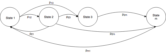
The most distinctive image associated with markov chains is probably that of the transition probability graph, which is simply a graphical way of representing the transition probability matrix.
About states: a state is a summary of the effects of the past in the future of some process. Because the chain verifies the markov property, a state must include all relevant information from the past. Suppose we’re visiting a zoo and decide which animal to visit next based only on the last animal we visited - in this case, each state need only include information about the last animal visited. Suppose now that we decide the next visit based on the last animal visited and also on whether it was day or nighttime when we visited it - then each state must include information about the last animal visited as well as whether it was day or nighttime during that visit. The point here is that the definition of the states in a markov chain is entirely dependent on the problem at hand. We consider only problems where the state space is discrete.
Defining the state space is crucial to setting up the model, and I suspect that, in practice, this will be more difficult than what this and the book’s simple examples let on.
In any case, given that we have a markov chain model in place, three questions are of interest when studying markov chains:
-
what does the system look like after a finite amount of time?
-
how does the system behave once it reaches an equilibrium? (steady-state behaviour)
-
how does the system behave until it reaches an equilibrium? (transient behaviour)
State after a finite amount of time
Given a markov chain model, a basic question is what is the probability of a particular sequence of future states. This is just the multiplication of the transition probabilities along that path. A simple example:
Given some initial state, the probability that the system will be in a certain state after $n$ timesteps is simply the sum over all possible paths that lead to that end. By the markov property, at each state along the path this probability will depend only on the previous state but not on the others before that. This means that we can write this probability, which we call the n-step transition probability, as a recursive law:
with $r_{ij}(1) = p_{ij}$. This is the Chapman-Kolmogorov equation.
It is useful to introduce some classification of states:
-
accessibility: a state $j$ is accessible from another state $i$ if $r_{ij} > 0$ for some $n$.
-
recurrency: a state $a$ is recurrent if, for all states $b$ that are accessible from $a$, $a$ is also accessible from $b$; in plain words, $a$ is recurrent if it’s possible to get back to $a$ no matter what transition out of $a$ occurs.
-
transiency: a state $t$ is transient if it isn’t recurrent, meaning that there exists some state that is accessible from $t$ but $t$ is not accessible from that state.
-
absorption: a state is an absorbing state if the only its only accessible state is itself. Meaning that if you get there, you’re not leaving.
-
recurrent class: a set of recurrent states that are accessible from each other is a recurrent class, or simply a class. Also, no state outside the class is accessible from a state within the class. This means that a class behaves like an absorbing state.
-
periodicity: this applies only to classes. A class is periodic if there exists some $n$ for which $r_{ij}(n)=0$, for some $i$,$j$ in the class. Conversely, a class is aperiodic if there exists some time $n$ such that $r_{ij}(n)>0$ for every $i$ and $j$. Another definition is that a class is periodic if its states can be grouped into disjoint subsets such that all transitions from one subset lead to the next subset. Intuitively, this just means that if a class is periodic then its transitions will oscillate between some subsets.
In this figure:
-
all arrows represent non-zero transition probabilities;
-
multiple states are accessible from each other. For example, c1 is accessible from t and c2; ap1 is accessible from ap2, ap3 and t; ap3 is accessible from ap1, ap2 and t; and t is not accessible from any state.
-
state a is absorbing: once you get there, you stay there;
-
state t is transient: once you get out of there, you don’t come back;
-
states ap1, ap2 and ap3 form an aperiodic class;
-
states c1 and c2 form a periodic class.
A neat summary of relevant properties regarding markov chains, shamelessly copied from the book:
-
a markov chain can be decomposed in one or more recurrent classes, plus possibly some transient states.
-
a recurrent state is accessible from all other states in its class, but not from any state in other classes (in can be accessible from transient states).
-
a transient state is not accessible from any recurrent state.
-
at least one recurrent state must be accessible from any given transient state.
Recurrent classes are the objects of interest when studying long-term behaviour of markov chains. This is because we’ll necessarily end up in a recurrent class: either we start at a recurrent state, meaning no state outside its class is accessible, or we start in a transient state, meaning we’ll eventually end up in a recurrent state.
Long-term, a.k.a. steady-state, behaviour of markov chains
When considering long-term behaviour we can limit our analysis to the case of a chain with a single recurrent class. This is because if there are transient states, we will necessarily end up in a recurrent class, so they don’t matter for the long term; and if there are multiple recurrent classes, we’ll still necessarily end up in a single one of them (and stay there) so we don’t need to consider all of them.
Moreover, if the single class is periodic, its state will oscillate between one or more subsets, meaning that its long-term behaviour depends on the initial state and does not converge to any value.
That being said, if we consider only markov chains with a single recurrent aperiodic class, then it so happens that the probability $r_{ij}(n)$ of being at state $j$ approaches a limiting value as $n\to\infty$, which is independent of the initial state $i$; on top of that, the $\pi_j$ are unique. This is the steady-state convergence theorem which, according to the authors, is “the central result of markov chains theory”.
A condensed version of the steady-state convergence theorem states that, given a single recurrent aperiodic class, the states $j$ are associated with steady-state probabilities $\pi_j$ that have the following properties:
The steady state probabilities form a probability distribution called the stationary distribution of the markov chain. They are stationary because if at some point $\mathbf{P}(X_k=j)=\pi_j$, then $\mathbf{P}(X_{k^\prime=j})=\pi_j \,\, \forall k^\prime>k$, meaning that probability stays the same regardless of future transitions.
These probabilities have an intuitive interpretation as long-term frequencies, i.e. $\pi_j$ can be interpreted as $\lim_{n\to\infty} \frac{v_{ij}(n)}{n}$, where $v_{ij}(n)$ is the number of visits to state $j$ within the first $n$ steps, starting from state $i$. Similarly, the frequency of transitions from state $j$ to state $k$ will be $\pi_j p_{jk}$, which is also fairly intuitive. Given this, then the balance equations also have a neat intuitive interpretation: $\pi_j$ is simply the sum of the expected frequencies of transitions that lead from any state to $j$.
Recall that we’re assuming finite-state markov chains. If we allow for infinite states, then the chain may never reach steady-state.
Transient, a.k.a short-time, behaviour of markov chains
We said earlier that transient states are irrelevant when considering long-time behaviour; that is of course not the case when considering short-term behaviour. We also established that a markov chain contains at least one recurrent class and possibly some transient states. We know that the system will eventually end up in the class, but we’re interested in understanding its behaviour until that happens; this means both knowing which recurrent state is entered and how long it takes until that happens. Of course, this is only relevant if the system starts in a transient state - if not, then we’re already in some class and back to the long-term situation.
For the purpose of understanding the chain’s behaviour until a class is encountered, we can consider every class to be a single absorbing state - this just means that we don’t care what happens once the class is reached, since we know the system can’t come out of it. If we fix some absorbing state $s$, we define the $a_i$ as the absorption probability that state $s$ will eventually be reached given that we start in state $i$. This means that we can find the absorption probability for state $s$ by solving the following system:
This makes sense: $a_s=1$ just means that the probability that we’ll end up in state $s$ given that we start there is $1$, which comes directly from the definition since it is an absorbing state; likewise, if we start at some absorbing state other than $s$, we’ll never leave it. If we start at a transient state $t$, then the absorption probability is just the absorption probability of all states accessible from $t$ times the transition probability from $t$ to that state. Reasonable enough. Conveniently, like the Chapman-Kolmogorov equations, the absorption probability equations have a unique solution.
This addresses the question of finding out which state we’ll end up in; there’s also the question of how long it will take to get to any one absorbing state. We define $\mu_i$ as the expected time to absorption starting from state $i$. We can obtain these by solving:
Again this is sensible enough: $\mu_{\text{recurrent state}} = 0$ just means that if we start on a recurrent state, we take 0 timesteps to get to a recurrent state. If we start in a transient state $t$, then the time to absorption is the time to absorption of all states accessible from $t$ times the probability that we’ll transition from $t$ to that state - plus one, since we still need one timestep to get to one of those accessible states.
We can exploit the same idea to find the mean first passage time, meaning the expected time to reach a certain state (rather than any recurrent state). This amounts simply to setting that state alone as an absorbing state and leaving all other states as transient states. In other words, if we focus on state $s$ and denote $t_i$ the mean first passage time from $i$ to $s$, then $t_i$ is obtained from the same equations we use to get the expected time to absorption:
What if now we want to find out how long it takes for us to get back to state $s$, given that we start out there? This is what we call the mean recurrence time of state $s$ and denote by $t_s^\ast$, which can be obtained by again exploiting the same idea:
which I think is quite intuitive - just the same as before, but starting on state $s$ rather than $i$. Note that if $s$ really is an absorbing state, then $p_{ss}=1$ and $p_{sj}=0$ if $j\neq s$, meaning that $t_s^\ast = 1$. This makes intuitive sense - if we’re at an absorbing state already, the mean time to get back to it is 1 timestep, meaning we get right back to it on the next transition.
Continuous-time markov chains
So far we have discussed only discrete-time markov chains, meaning that the time between transitions is fixed (1 timestep). We now consider the case where transitions can happen continuously. The time between transitions is then a continuous random variable, rather than a constant. Continuous-time markov chain models are relevant in contexts where events of interest are described as Poisson processes. An example is the number of active calls in a call center where the incoming calls are modeled as a poisson process.
We introduce two assumptions to handle the continuous case:
-
if the current state is $i$, the time until the next transition is exponentially distributed with parameter $\nu_i$ which is independent of past states and of the next state, i.e. depends only on state $i$.
-
if the current state is $i$, the next state is $j$ with a probability $p_{ij}$ which is independent of past history (the markov property we already knew) and also independent of the time until the next transition.
This is a neat formulation because it separates the sequence of states and the time for transitions. As an immediate consequence, the sequence of states obtained after successive transitions is a discrete-time markov chain - we call it the embedded markov chain. Note that this is different from describing the continuous-time markov chain as an approximate discrete-time markov chain, which I discuss further ahead.
Let’s introduce a notation shortener for the history of the process until the $nth$ transition:
In the discrete case we had:
In the continuous case we introduce the time component:
Using the mean of the exponential distribution, the expected time to the next transition is $\frac{1}{\nu_i}$. Hence $\nu_i$ can be thought of as the frequency of transitions out of state $i$, and is cumbersomely called “transition rate out of state $i$”. Out of these, only $p_{ij}$ will be into state $j$, and so we define the transition rate from $i$ to $j$ as $q_{ij} = \nu_i p_{ij}$.
Given the transition rates, we can provide an alternative description of a continuous markov chain by observing that, for a starting state $i$ and small time units $\delta$, the state after $\delta$ time units is $j$ with probability $q_{ij}\delta$. This is a bit of a rough description, but this is the key idea: instead of transition probabilities we have transition rates, and so to obtain probabilities again we have to multiply by some time.
Using this approach, the questions of interest that we talked about before can be addressed by relying on this approximation, i.e. by replacing $p_{ij}$ with $q_{ij}$. One example is the steady-state behaviour situation: the balance equations, which in the discrete case were
become, in the discrete approximation of the continuous chain,
which just means that the expected frequency of transitions out of j to all other states is the same as the expected frequency of transitions into j from all other states.
A final interesting point is that, for a given continuous chain, the steady-state probabilities of its discrete approximation and of the embedded chain are in general different - the reason for this is that if the frequency of transitions out of state 1 is lower than that of state 2, i.e. if the system spends more time in state 1 than state 2, then it is more likely to be found in state 1 in the long-term. Since the embedded chain ignores transition times, it does not capture this property.
Literal textbook example
To wrap this section up I’ll describe an example that seems to be canonical given how often it shows up in the book’s examples and exercises: birth-death processes.
A birth-death process is some process that can be expressed as a linear markov chain where the only allowed transitions for state $i$ are to states $i-1$, $i$ or $i+1$ (except for the endpoints, where $i-1$ or $i+1$ are not allowed, i.e. the chain is not cyclical). The transition matrix for this process has a fat diagonal with 3 elements per row and zeros elsewhere. Transition probabilities from state $i$ to state $i+1$ are denoted $b_i$ and called birth probabilities; similarly, transition probabilities from state $i$ to $i-1$ are denoted $d_i$ and called death probabilities. Self-transition probabilities are simply $p_{ii}=1-b_i-d_i$. These processes “arise in many contexts, especially in queueing theory”.
In this context, the steady-state behaviour can be simplified because the only allowed transitions are from neighbouring states; the balance equations become the local balance equations:
which simply reflect the intuition that, if the system is stationary, the probability of a transition out of every state must equal the probability of a transition into that state.
In the continuous case, the local balance equations become simply
What I realized I need to improve
Two skills came up recurrently while working through this subject: series and demonstrations. In both cases, I realized I understand them worse than I expected. Regarding series, I remember I never did properly learn them as an undergraduate, and it really showed - problems as simple as summing a geometric series required looking up the solution. While I don’t see this skill as an urgent need, it is definetely something worth improving and a candidate for future work.
As for demonstrations, I realized I could frequently grasp the general idea of why some statement was or was not valid but failed to adequately articulate the proof. More so than series, I think this would be a skill worth working on since it would help me improve on my mathematical thinking and on how to approach new problems.
Also I clearly need to do a crash course in html and css to at least be able to center those figures.
Take-aways
A couple of noteworthy take-aways from this process:
-
stronger habits: my number one goal with this endeavour was to forge a learning habit by consistently dedicating time to learning some topic. I feel this goal was fully achieved, and that I now have a habit that I can lean back on to find time to work on skills I find relevant. In addition, I learned a lot about what helps create a habit. From this point of view this process was very much worthwhile.
-
comfortable with Markov chains: my number two goal was to learn more about Markov chains, to a point where I would feel comfortable discussing them with someone else or considering them to solve some real-world problem. I feel that this goal has also been achieved, even though I struggled with a few of the demonstration problems.
Where to go from here
There are two subjects which are related to markov chains and I would like to understand in greater detail: hidden markov models and markov chain monte carlo methods. More generally, I feel that I need to learn more about random processes.
Figures created with draw.io.